HiPERCAM
Because HiPERCAM is optimised for high time resolution, there are a number of peculiarities to it’s use. You should read this document in full before creating a phase II submission.
HiPERCAM is a deceptively complex instrument to use. Even if you are already familiar with HiPERCAM, we strongly recommend using the Checklist to check your setups before submission.
The primary consideration when observing with HiPERCAM is to realise that its frame-transfer CCDs have no shutter. Instead, an image is rapidly moved into the storage area, which begins a new exposure in the image area. The image continues to expose whilst the storage area is reading out. As a result there is very little deadtime between exposures. However, one cannot start a new exposure whilst the storage area is being read out; this sets a minimum exposure time equal to the time needed to readout an image.
Obtaining a desired exposure time involves selecting a readout mode (binning/windows), which sets the minimum possible exposure, and optionally adding a delay to get the desired exposure time and cadence.
Cadence / exposure time
Therefore, the first thing you should decide is what cadence your science requires. The longer it is, the easier things tend to be. A key feature of HiPERCAM, if you are trying to go fast, is that there is a trade off between how fast you can go and how much of the CCDs you read out and/or what binning you use. If you try to go very fast, e.g. less than 3 second cadence, you will need to use Windowed mode, or bin the readout. For extremely fast observations (more than 10Hz frame rate) there is a special option (Drift mode) to reduce readout overheads further. For observations where even shorter exposures are needed, there is a special mode (Clear mode), which can be used at the expense of dead time overheads. Therefore, the exposure time can define multiple other aspects of the setup.
For any given setup (binning, window sizes and positions, readout mode), there is an
absolute minimum exposure time which is set by the time taken to
readout the storage area. One can expose for longer than
this minimum by adding an arbitrary “exposure delay”; this is a key
parameter of the hfinder setup. So perhaps your setup can be
readout in 3 seconds, but for reasons of signal-to-noise perhaps you
add 7 seconds exposure delay. Then your exposure time (and cadence, as
dead time is negligible in this case) will be 10 seconds. If you set
the exposure delay to 0 however, your exposure will be 3 seconds and
you wouldn’t be able to go faster without altering the setup.
If your objects are not variable, then, as usual for CCD imaging, you should consider:
the signal-to-noise you need (
hfinderwill provide a summary and there is an online calculator that gives full details),the avoidance of saturation of your target and possibly comparison stars,
allowing enough time for the sky background to dominate over readout noise for faint sky-limited targets especially, and
whether you want to divide up exposures perhaps for dithering the position, or to enable exploitation of brief periods of best sky conditions, e.g. seeing.
Note
An exposure time of 30 seconds, binned 2x2, will be sky-noise sky-limited (sky noise ~ 3x readout noise) in the u-band even in dark time. For 1x1 binning the same ratio is reached in 120 seconds. There is not much to be gained in using longer exposure times than this. We do not recommend using exposure times longer than 120 seconds when binned, or 240 seconds binned 1x1.
For time-series observations of variable targets, considerations 1, 2 and 3 may still apply, but you also need to decide on the timescale you aim to sample. Because of the dependence of the minimum exposure time on the setup described earlier, this timescale may drive later decisions. For instance, HiPERCAM’s full frame, unbinned readout time is about 3 seconds. If you need to go faster than this, you will need to bin or window. This is a trivial but common example of the interplay between exposure time and CCD setup.
Spatial sampling / binning
It is quite common to see setups with 1x1 binning selected. However, in most cases 1x1 binning is not the best choice, and sometimes it is a very bad choice. There are three reasons for this:
HiPERCAM’s native unbinned pixel size on the GTC is just 0.081 arcseconds, which significantly oversamples all but the very best seeing. Thus if you bin 2x2, 3x3 or even 4x4, you might not lose much resolution at all.
Binning substantially reduces the amount of data. This can allow you to readout the CCD faster. This could mean for example that you can read the entire CCD binned, whereas you would have to sub-window if unbinned. Reading the whole CCD means there are more comparison stars available, makes observing easier, and ensures that objects are not too close to the edge of the readout windows.
Binning reduces the impact of readout noise. CCD binning occurs on chip before readout, so readout noise is incurred per binned pixel, not per native CCD pixel. This can have a very large impact on your data, depending upon target and sky brightness. You should, if possible, define a setup that ensures that the peak target counts per binned pixel are substantially in excess of \(R^2 G\) where \(R\) is the RMS readout noise in counts (ADU) and \(G\) is the gain in electrons per ADU. For HiPERCAM this means one wants if possible at least 100 counts/pixel at peak, and preferably higher than this. Note this does not apply for long exposures where the sky noise dominates. If the sky counts are greater than 100 counts/pixel, then there is less to be gained since binning increase the target and sky counts per pixel by the same factor, but when going fast, the sky can often be quite low level (especially in CCDs 1, 2 and 3, i.e. ugr). This means it can make sense sometimes to use very large binning factors when going fast and sky noise is low. It is this sort of case when binning can quite dramatically improve your data, and if you are not worried about spatial resolution at all, 8x8 or even 16x16 binning might make sense.
Binning has downsides of course; resolution is the obvious one. If you need to exploit good seeing, then you may not want to go beyond 2x2 binning (0.162 arcseconds/pixel). The other effect is that you are more likely to saturate the CCD. However, points 2 and 3 above mean that more often than not you should bin, and you should think twice before simply selecting 1x1. To understand more about how one guard against readout noise, see the section below on condition-tolerant setups.
Note
The binning is the same for all CCDs. There is another option for
accounting for differences between CCDs. See the discussion of nskips
below.
Note
The peak counts per binned pixel are displayed by hfinder if
you set the correct magnitude for the target and selected
filter. This is a very good way to judge your setup.
Readout modes
Outputs
HiPERCAM has four separate outputs, or channels, per CCD. The division between these
outputs is clearly shown in the FoV in hfinder.
Warning
Each output has a different gain and bias level. You must avoid putting critical targets on the boundary between outputs.
Windowed mode
To enable higher frame rates, HiPERCAM can use one or two windows per output. Since there are four outputs, we refer to window quads to define window settings. You can enable windowed mode by selecting Wins for the Mode option in the instrument setup panel.
A window quad is defined by the x-start positions of the four quadrants, the size of the windows in x and y, and a y-start value. All windows in a quad must be the same shape, and all share the same y-start value. Increasing y-start moves the windows in from the edges of the CCD towards the centre.
If there are two window quads, they cannot overlap in y.
Synchronising windows
If on-chip binning is enabled, it is possible to define windows that do not align with the boundaries of the binned pixels. This means that one cannot crop binned, full-frame calibrations (such as bias frames) to apply to the windowed data. If windows are not synchronised in this manner, the Sync button will be enabled. Clicking this will align the windows with the boundaries of binned pixels.
Warning
Unless you have requested special calibrations for your data, e.g binned sky flats, you should make sure your setup is synchronised.
Clear mode
Sometimes extremely short exposures are needed, even with full frame data. Bright standard stars would be one example. It is possible to clear the image area of the CCD, just after the storage area is read out. This allows exposure times as short as 10 microseconds. These short exposures come at the expense of efficiency, since the charge accumulated whilst the storage area was reading out is lost.
For example, if the storage area takes 2s to read out, clear mode is enabled and the exposure delay is set to 1s, then an image would be take every 3s with a duty cycle of 30%.
As a result, if the user needs short exposure times to avoid saturation, or if short exposures are needed for science purposes, then it is often preferable to use a faster readout speed, Windowed mode or Drift mode to achieve this without sacrificing observing efficiency.
Clear mode is enabled by selecting the Clear checkbox.
Drift mode
Drift mode is used to enable the highest frame rates. Instead of shifting the entire image area into the storage area at the end of each exposure (a process that takes 7.8 milliseconds), only a small window at the bottom of the CCD is shifted into the storage area. This minimises the dead time involved in shifting charge to the storage area and allows frame rates of ~1 kHz for relatively small windows.
In drift mode, a number of windows are present in the storage area at any one time. At the same time, any charge in pixels above the windows is eventually clocked into the windows, and becomes part of that frame. To prevent bright stars from contaminating the drift mode data, a blade is inserted into the focal plane, blocking off most of the image area of the CCD. Because the windows in drift mode spend longer on the chip, they accumulate dark current; drift mode should only be used for frame rates faster than ~10 Hz as a result.
In drift mode, only two windows are read out (at the bottom of the CCD). Clear mode is not possible in combination with drift mode.
Diff-Shift
After transfer to the storage area, both windows have to be clocked horizontally to reach the readout register. Therefore the fastest speeds are obtained when the windows are in the corners of the CCD. If the windows are moved in from corners, it is best to move them inwards an equal amount, since otherwise the window on the side closest to the readout register will have wait until the other window reaches the readout register, slowing down the frame rate.
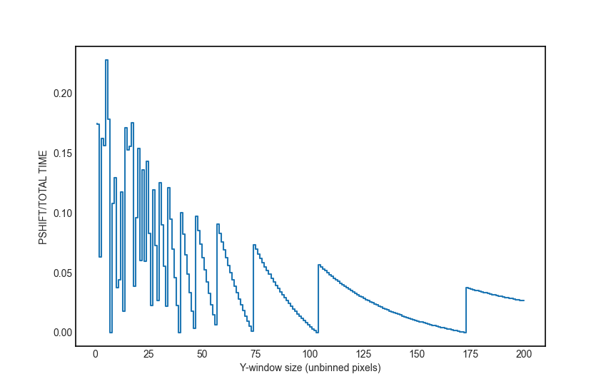
Pipe-Shift
Another effect that can improve the efficiency of drift mode is choosing the y-size of the window. When the vertical height of the storage window does divide perfectly by the y-size of the windows, an additional number of vertical clocks, called a “pipe-shift” is introduced, so that the drift windows are evenly spaced within the storage area. It is therefore best to use window y-sizes that divide evenly into the storage area height. These y-sizes are called “magic numbers”. The plot below shows the fractional contribution of the pipe-shift to the total readout time, as a function of the window y-size. Choosing your window size to minimise this contribution will maxmise frame rate and duty cycle.
Details
For more information about drift mode, see the ULTRACAM instrument paper and it’s appendix.
Exposure multipliers (nskips)
The instrument setup will determine the exposure time and cadence of your data. It is unlikely that this exposure time will be optimal for your target in all bands. Many objects will need longer exposures at the blue or red extremes. HiPERCAM supports exposure multipliers. These allow a CCD to be readout once every N exposures, and can be changed in the fields labelled nu, ng…
For example, consider a target of magnitude g=20, u=20. In one second, and with 4x4 binning,
hfinder reports 262 counts at peak in g, but only 40 in u, so the u band is below the
readout threshold discussed earlier. If one is happy instead to use 3 second exposures in u,
then this can be fixed by setting nu = 3, which will mean the u-band CCD will read out every
three frames.
Warning
The peak counts reported by hfinder do not account for the
nskip values, so you need to take them into account when judging the
peak count level. You should check values for all CCDs.
Note
It is usual to run with at least one of the nskip values set = 1, so that at least one CCD is read out every time. One could in principle set values like 5,4,3,2,2,3 to deliver fractional exposure time ratios. It is not advised though, because (i) there should be enough dynamic range between readout-limited data and saturated data that integer ratios are OK, (ii) each CCD is always readout each cycle, but nskip-1 of the readouts are dummy readouts producing junk data. Thus with a minimum nskip of 2, at least 50% of the data for each CCD is junk. The software is designed to ignore this, but it is wasteful of disk space. A set of nskip values like 9,6,3,3,3 i.e. with a common divisor, is a mistake as it could be changed to 3,2,1,1,1 and the exposure delay adjusted to triple the cadence. This would deliver identical data but cut down the overall size by a factor of 3.
Comparison stars
If you have to use windows, their exact definition very much depends upon the field of your target. At minimum one should include at least one and preferably two or more comparison stars if possible. They should be brighter than your target. It often helps to have one that is quite significantly brighter for the u-band, particularly for blue targets, as the average comparison is red, and it can quite often be the case that a comparison that is moderately brighter than the target in the redder bands is scarcely visible in u. Remember one does not need to use the same star as comparison in each filter and its OK for a comparison used in u to saturate in all other bands, as long as there is a backup comparison for those bands.
Warning
Avoid setups in which a bright star is on the same column (i.e. same X position) and same quadrant as a faint target. This is because the frame transfer leaves a low level vertical streak that could be problematic if there is a very bright star lined up with your target.
Warning
Do not place your target or comparisons close to the half-way point in either X or Y in full frame mode because the HiPERCAM CCDs are read out at the 4 corners and you risk your target being divided across multiple Outputs.
Using COMPO for better comparison stars
Sometimes there are no good comparison stars in the field of view. To address this issue, HiPERCAM is equipped with a COMparison PickOff (COMPO).
COMPO works by using a small pick-off mirror on a rotating arm to capture light from a star outside the field of view. The light is then fed into an injection arm which can optically place the light from the star into one corner of the CCD, effectively changing the on-sky position of the star. The pickoff and injection arms have a field of view of 24 arcsec.
The injection arm will vignette the corner of the CCD in which is is placed.
Use of COMPO is enabled using the COMPO checkbox. This brings up a small COMPO widget that allows one to set the position of the injection arm and the rotation angle of the pickoff arm. The current COMPO setup is also displayed, as shown below.
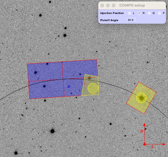
The pickoff and injection arms are shown in yellow. The rectangular region shows the vignetted area, and the circle shows the field of view of the arms. The black line shows the path the pickoff arm will take as it rotates.
By changing the telescope PA and pickoff arm angle, you can place your desired comparison star within the field of view of the pickoff arm. The position of the injection arm is selected using the radio buttons. The options available are:
L |
Position arm in lower left corner of CCD |
R |
Position arm in lower right corner of CCD |
G |
Position injection arm over the guide camera. |
P |
Park injection arm out of the FoV (also parks pickoff arm). |
By positioning the pickoff arm over a bright star and selecting G for the injection arm, compo can be used as an off-axis autoguider for long exposures.
Miscellaneous settings
The remaining settings you can change are described below:
- Num. exposures
The number of exposures to take before stopping. Most HiPERCAM users will want to take a continuous series of exposures and stop after an alloted time. In which case this field should be set to 0. If you want your OB to have a specific duration, the correct number of exposures is found by dividing the time required by the cadence reported by
hfinder.- Readout speed
Fast readout speed reduces the minimum exposure time in full-frame readout from 2.9s to 1.2s. This comes at the expense of increased readout noise. The impact of this on the S/N of your target is shown in
hfinder.- Fast clocks
Users wanting the ultimate in high speed performance can enable this option. This increases the rate at which charge is clocked in the CCDs. It will have an impact on charge transfer efficiency. As of today, this impact has not been well characterised, but we do not think it is serious.
- Overscan
Enable the recording of the overscan regions at the left and right edges of the chip. Can be useful if precise measurement of the bias in each frame is needed. This can be useful for the highest levels of photometric precision. If the bias level is wrong, the sky background (and thus the estimated errors on the photomtry) will be wrong, so consider this option for, e.g. exoplanet transit observations.
Autoguiding
HiPERCAM is mounted on the FC-G rotator. This instrument port has no built-in autoguider. Autoguiding is therefore provided by the science instrument itself. There are two options for autoguiding: guiding using the science images themselves, or using COMPO as an off-axis guider.
Autoguiding using the science images
For relative short exposure times (less than around 60 seconds), the tracking of the telescope is
adequate to provide sharp images. The best option for guiding is therefore to use the position
of bright targets in the science images to correct for any drift in the telescope pointing.
This requires no setup using hfinder, and is performed by the support astronomer on the night.
Autoguiding using COMPO
For longer exposure times, the tracking of the telescope is not adequate to provide sharp images. Active autoguiding during a single exposure is required. For this purpose, COMPO can be used as an off-axis guider. This is enabled by selecting G for the injection arm and positioning the pickoff arm over your chosen guide star.
Note
Guide stars in the magnitude range (XX-XX) are most suitable for guiding.
Warning
Many extra-galactic observations use a combination of long exposures, and dithering to allow accurate background removal. This is possible with COMPO autoguiding, but requires that the offsets between dither positions is small. The FoV of the pickoff mirror is 24 arcseconds, so no offset position should be further than 10 arcseconds from the central position.
In principle it would be possible to supply a telescope PA and pickoff angle position for each dither position, to ensure the guide star is always visible when larger offsets than 10 arcsecs are required. However, this mode is not currently supported (as of Summer 2023).
Dithering the Telescope
It is possible to dither the telescope between frames. This can be useful if, for example, you want to make a flat-field directly from the night sky observations themselves. Clear mode is always enabled when dithering the telescope, to avoid trails from bright stars appearing in the image.
The overheads involved in moving the telescope mean that there is little point in using any mode other than full-frame readout with this option.
If you wish to dither the telescope, check the Nodding checkbox. You will be prompted for a plain text file specifying the offset pattern you require. The format of this file is a simple list of absolute RA, Dec offsets in arcseconds as shown below:
0  0
0  20
20 20
20 0
0  20
This offset pattern will be repeated until your exposures are finished. hfinder
will estimate the impact of nodding on your cadence and overal signal-to-noise.
If you wish to visualise the dithering pattern on the sky, pressing the n key
will cycle through the dithering pattern.
Condition-tolerant setups
If you are sure that your target will only be observed with seeing close
to 1.2” and during clear conditions, you’ll have a relatively easy job
defining a setup. Much more difficult is if the seeing could be
anything from 1.2 to 2.5”, the reason being that the peak counts could
vary by more than a factor of 4. The key point here is probably the
binning. It should definitely be at least 4x4, and arguably 6x6 to
8x8, otherwise you could end up swamping the target with readout noise
during poor seeing. One way to think about readout noise is as the
equivalent of \(R^2 G\) counts from the sky in each binned pixel.
If you use 1x1 rather than 8x8, you have just increased this
contribution by a factor of 64. Sometimes this won’t matter; sometimes
it will be a disaster. As always, the thing to do is try different
setups and seeing values in hfinder, and the key to using it is to
understand the signal-to-noise values hfinder reports.
S/N vs S/N (3h)
If you look at hfinder you will see two values of
signal-to-noise. One, “S/N”, is the signal-to-noise of one frame. The
other, “S/N (3h)”, is the total signal-to-noise after 3 hours of
data. The latter can reach unrealistically large values (e.g. 14584 in
the screenshot) which are meaninglessly high in practice,
nevertheless, the “S/N (3h)” value is one of the best ways to compare
different setups as it accounts for the issue of shorter exposures
versus a larger number of exposure and also deadtime. One way to find
a condition tolerant setup is to find one where the “S/N (3h)” value
does not respond dramatically to the exact setup.
As an example, consider a star of g=18 being observed at high speed in dark time, seeing 1”, airmass 1.5. With 1x1 binning and windows of 92x92, I find a cadence of 0.101, a duty cycle of 92.3% and an “S/N (3h)” value of 3772. This is not obviously bad, but the peak counts are listed as just 10! This will be heavily read noise affected. This becomes obvious if I add 0.1 seconds to the exposure delay giving 0.201 cadence, 96.1% duty. The S/N (3h) becomes 5306. That’s the equivalent of \((5306/3772)^2 = 1.98\) times longer exposure, but the duty cycle only increased by a factor of 1.04. The large improvement is because I have halved the number of readouts.
What if I still want the 0.1 seconds? Then I should bin. So, the same target and conditions, but now with binning 4x4 and cadence 0.1 seconds, I find again a 92% cadence, but the S/N (3h) value is now 9970 and I have gained a factor of 7 in effective exposure time! So the first setting was really a disaster. To judge how much further there is to go, I make the cadence 10 sec, and find S/N (3h) = 13400, but of course 10 seconds may be unacceptably long, but still it shows what one should be aiming at.
What about the impact of seeing? If I set seeing to 2”, the S/N (3h) for the 4x4, 0.1-sec mode drops to 6265, equivalent to dropping the exposure down by a factor 0.4. The 1x1 version drops to 1937, equivalent to just 0.26 of the exposure, so not only is it a bad setup, but it gets worse more quickly.
Warning
These are not small effects, and you need to think about them for all CCDs. CCD 1 (the u-band) is almost always the most sensitive of all to readout noise issues. “nskip” is your friend then. If possible try to find the sweet spot between being well above the readout noise, but not in danger of saturation. Peak counts (factoring in any nskips) from 1000 to 15000 are what you might want to aim for, although they won’t always be possible.
Checklist
Have you chosen your binning to give the spatial sampling you need? 1x1 binning is very rarely the best choice, and can increase readout noise dramatically. HiPERCAM’s native pixel size is only 0.081” on the GTC, so you can resolve typical seeing discs with 3x3 or 4x4 binning.
Could your setup lead to saturation in good seeing? If so, is there leeway for the observer to reduce the exposure time (a relatively easy change) without the need to change the setup (time consuming)?
Have you checked the peak counts per pixel in all CCDs, especially CCD 1 (u-band)? Is it comfortably above readout? (100 counts or more). The nskip parameters (nu, ng, nr, ni, nz) may help.
Is your target away from the edges of the CCD outputs in both X and Y to avoid a split readout and consequent data reduction problems?
Have you ensured that no very bright objects are aligned along the Y direction and in the same quadrant as your target?
For blue targets, have you included a bright comparison star (if available) for the u-band, even if it looks too bright for the griz bands?
For variable targets, have you considered the impact of the full range of their variability in terms of possible saturation or readnoise?
If your exposure times are long (more than approx 60 seconds), have you enabled the use of COMPO, and positioned the pick-off mirror over a suitable guide star?
Is the duty cycle of your setup what you expect? For most observations it should be above 95%.
Is your setup tolerant of the full range of conditions you have specified for it? Variations in seeing especially, can cause dramatic variations in peak count levels and may veer you towards either saturation or readout noise limitations.
Does the product of the number of exposures and the cadence match the times you want to follow your target?
Do you need to dither your observations for optimum background subtraction?